Maxwell
A 2D FDTD solver for Maxwell's equations
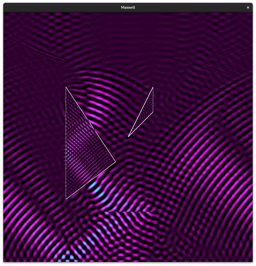
Maxwell is a real-time electromagnetic field simulator written in C. It solves Maxwell’s equations on a 2D grid using the finite-difference time-domain (FDTD) method, with GPU acceleration via OpenCL and live visualization via OpenGL.
The FDTD method discretizes both space and time, updating electric and magnetic field components on a staggered Yee grid at each timestep. This naturally captures wave propagation, reflection, refraction, diffraction, and interference – all emerging from the underlying differential equations without special-case handling.
Features
- GPU acceleration via OpenCL, with automatic CPU fallback
- Boundary conditions: natural, perfect electric conductor (PEC), and perfectly matched layers (PML) with configurable absorption profiles
- Arbitrary sources coupled to any field component – sinusoidal excitation with user-defined frequency and phase
- Material regions with user-defined permittivity, permeability, and conductivity (triangles and circles)
- Live rendering with real-time OpenGL visualization and multiple visualization modes
- Interactive controls – pause/resume, reset, toggle material boundaries, cycle visualization functions
How it works
The simulation evolves the electromagnetic field by alternately updating the electric field $\mathbf{E}$ and magnetic field $\mathbf{H}$ using the curl equations:
$$\frac{\partial \mathbf{H}}{\partial t} = -\frac{1}{\mu} \nabla \times \mathbf{E}$$
$$\frac{\partial \mathbf{E}}{\partial t} = \frac{1}{\epsilon} \nabla \times \mathbf{H} - \frac{\sigma}{\epsilon} \mathbf{E}$$
In 2D (TE mode), this reduces to updating three field components ($E_x$, $E_y$, $H_z$) on a staggered grid. The spatial derivatives become finite differences, and the time evolution uses a leapfrog scheme where $\mathbf{E}$ and $\mathbf{H}$ are evaluated at alternating half-timesteps.
The PML boundary condition works by introducing a fictitious lossy medium at the edges of the simulation domain. The conductivity increases polynomially from zero at the inner boundary to a maximum at the outer edge, absorbing outgoing waves with minimal reflection.
Configuration
Simulations are defined in plain text configuration files:
[Simulation]
Width 500
Height 500
Boundary PML 20 5.0 3
ComputeOn GPU

[Sources]
SineLinFreq Hz 250 250 0.05 0

[Materials]
Triangle 4.0 1.0 0.0 200 200 300 200 250 100