A Fluid that Computes

Wednesday, October 7th, 2026

Yesterday, 6 Oct 2026, OpenAI released an enormous corpus of math manuscripts on their GitHub. These results, some 700 and change, were grouped into a few hundred families. One of those families was universal computation in forced Navier-Stokes flows (family 376) – this is a collection of works having to do with demonstrating that viscous incompressible flows starting from rest perform universal computation under smooth external forcing. Of all the works they published, this was the group that most drew my attention. The idea itself is beautiful and has historically been a favorite of mine when discussing computation with people.Like whether you can embed a program in a distribution of masses and run it over its inputs by sampling gravitational trajectories! More generally, the power to choose an arbitrary potential landscape for a particle is sufficient to simulate a Turing machine (Moore, 1990).

Despite being aware that designing such a “machine” is in principle possible, I have never been made aware of any even mathematical (as opposed to truly physically-realizable) implementation under any regime (fluid or gravitational or otherwise). Moore’s 1990 work showed that “generalized shifts” are as powerful as Turing machine, and provides an embedding to a particle in a 3D potential.² However, Moore never actually provided any implementation. Later work by others in Euler flows³⁴ provided similar principled existence proofs but no actual implementations.

This work by OpenAI is remarkably interesting because it provides a general recipe to actually determine the forcing pattern required to implement an arbitrary program: a universal converter which turns any Turing machine into a table of instructions, and a routing theorem showing how a smooth flow can carry out all these instructions at once. Once we know the flow we want, the force doesn’t have to be designed at all – we just set pressure to zero in the equations and attain it for free from whatever makes the Navier-Stokes equations hold. This means we can actually sit down and build a computer this way. As far as I can tell, this is something that no one has done before. The aforementioned earlier works proved that such flows exist and even provided constructions in principle, but none were ever computed and run.

Inspired by this all, coupled with the recent flurry of postings of Claude Opus 5.5’s beautiful visual works, I decided to set to work alongside him attempting to see if we could not only implement OpenAI’s construction for a real meaningful computation, but also produce a visual render demonstrating how the machine functions.

As a target, we wanted to produce something that clearly wasn’t a stunt. A flow that drifts from “13 × 11” to “143” doesn’t really demonstrate anything, and neither does a lookup table. As such, we settled on the standard binary shift-and-add algorithm for multiplication: the same way it is done in hardware. We keep a running total \(A\), and start with multiplicand \(M\) and multiplier \(Q\). So long as \(Q\) has bits remaining, add \(M\) to \(A\) if \(Q\) has lowest bit \(1\), then double \(M\) and halve \(Q\). This setup requires all the typical machinery: memory, branching, arithmetic-with-carry, looping, and a halt condition. At four bits of input, this system stays small enough to watch every step, while still exhibiting every part of a recognizable computation.

Watch the computer run

Here’s the result of that work. Before explaining how it works, here’s what to watch for. OpenAI’s construction guaranteesThis is the main theorem (Theorem 4.1) of Incompressible Box Transport and Finite Computation, stated in Lean as balanced_three_stack_realization in BalancedThreeStack.lean. Strictly, we ran our own program in the theorem’s format rather than its general Turing-machine converter, and verified the same conditions exactly, so the guarantee carries over.¹ that the particle whose position encodes the machine’s state (the white speck) enters the golden detector volume on the left exactly when the program halts, and never before. Furthermore, its landing position within that volume encodes the answer to the computation. As such, be mindful of the position of the white particle as it transitions between the machine’s internal states, never entering the golden cube until the end.

Each of the 13 cubes in the video is one of the states of the machine, sort of like the line a program is currently on. The blue and violet cubes handle the upward sweep through the bits (where violet means the current bit of \(Q\) says to add to \(A\)), teal handles the return sweep, and the golden cube is the end detector. The glowing bands are the instructions themselves. Each one is a block of fluid, and each cycle of the machine lifts the block from its cube, stretches it, and sets it down in the next state’s cube. If the block’s destination is not yet free, it waits in a storage area overhead. The visible registers are not scripted either, rather they are decoded from the speck’s exact position each time an iteration completes. After the 53 cycles, the speck drops into the end container and its position encodes the answer to \(13\times11\) as \(143\).

How it works

We are able to do all this essentially thanks to being able to hold an unbounded amount of information in the position of a particle (that is, by representing its position to arbitrary position, we can record as much data as we need). For each component of the particle’s position, write it in base 27, and read the “digits” after the decimal as a stack of symbols, with the first digit on top. Popping a symbol off the stack means deleting that first digit, which is the same as multiplying by 27 and throwing away the whole-number part. Pushing a symbol on means shrinking by 27 and adding it in front. Each of the components becomes one of three stacks: \(R\) holds the bits of \(A\) and \(M\), paired up column by column so the adder can read both at once, \(J\) holds the bits of \(Q\), and \(L\) holds the columns currently being worked through, along with a record of every multiplier bit already used. Only the odd digits are used as symbols – the even ones are left empty as gaps, so that different symbols never touch and the flow always has room to work.

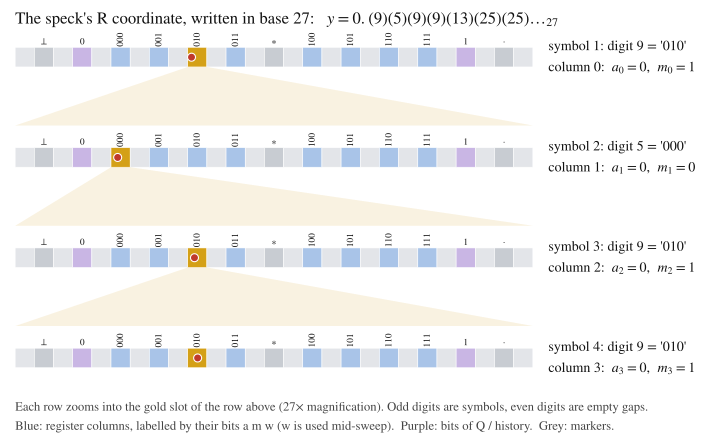
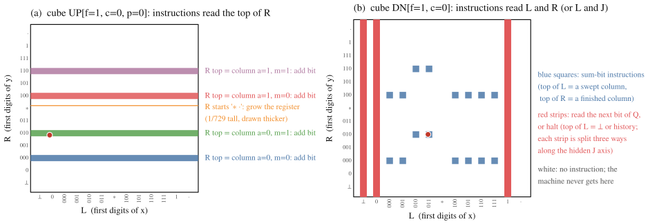
The whole-number part of the position – which of the 13 cubes the speck is in – tells us which line of the program the machine is on, and each line has a handful of instructions of the form “if the top of \(R\) is the column \((a=0, m=1)\), pop it, push its updated version onto \(L\), and go to the next line.” Every configuration an instruction applies to shares those same top symbols, and so they all sit together in one region of the cube: a thin band if the instruction reads one stack, or a small square if it reads two. Each cube is carved up into these regions, one per instruction, and the speck sits in exactly one of them. That region is the instruction it runs next.

Running an instruction then just means moving its region. The flow lifts the band out of its cube and sets it down in the next line’s cube, stretched 27× along one axis (a pop) and squeezed 27× along another (a push). Everything inside moves together as one piece, so the deeper digits – the rest of the memory – ride along untouched. This is exactly the stretching and turning of the bands in the video. Crucially, the force can’t know where the speck is, so it moves every region, every cycle: all 122 instructions, no matter the input. Everything else moving in the video is the program being applied to situations the machine isn’t in.

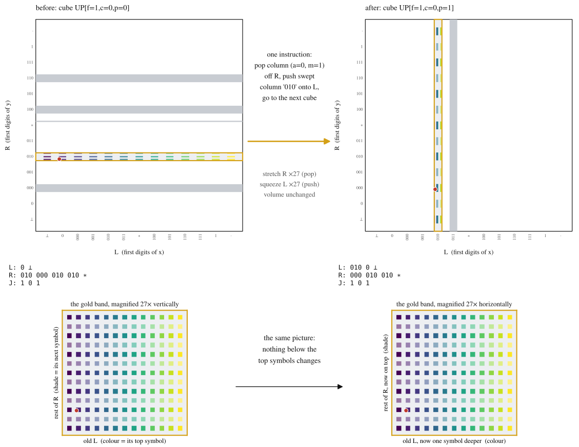
An incompressible fluid can only stretch a block if it squeezes it by the same factor elsewhere, so every instruction must remove exactly as many symbols as it adds. A fluid also can’t merge two blobs into one, so no instruction may destroy information. Ordinary addition does destroy information (you can’t recover \(a\) and \(c\) from \(a + c\)), so our multiplier uses a reversible adder⁵ and keeps each used bit of \(Q\) on a history stack rather than erasing it – an old trick from reversible computing.⁶

Is it really Navier-Stokes?

The forced incompressible Navier-Stokes equations are:

$$\partial_t u + (u\cdot\nabla)u = -\nabla p + \nu\Delta u + f, \qquad \nabla\cdot u = 0.$$

Around each moving region, the velocity is built as the curl of an explicit, smooth, localized vector potential. As such, it is divergenceless by construction, as well as switching on and off smoothly. It vanishes as well, outside a bounded region. Then comes the trick from earlier: set the pressure to zero and define the force as whatever is left over:

$$f = \partial_t u + (u\cdot\nabla)u - \nu\Delta u$$

The equations then hold exactly, at any viscosity. The force is fixed and smooth, repeating exactly each cycle. It depends only on the program. The same force multiplies all pairs of four-bit numbers at the same time (as the input only chooses where the speck starts, not anything about the global behavior of the force). Given that force, an energy argument shows this must be the only reasonable solution.

A warning: this computation cannot survive floating point. Each pop magnifies errors 27-fold, and a double-precision integration will lose the computation after only a few dozen cycles. As such, you must compute each position exactly.

Could a real fluid do this?

Nope. Definitely not. The complete machine state is encoded in the particle’s position. Our multiplication (and a small one, at that) goes twelve base-27 digits deep, which means that we are talking about precision on the order of \(10^{-17}\) against the cube side length. For a cube a meter across, that means accuracy much smaller than the size of a proton. Brownian motion alone scrambles things far more coarsely than anything even approaching that. And even in principle, there is no way to do error correction in a flow like this, due to volume preservation (there’s no way to squeeze a cloud back down to a point).

One trick you can try is to spend volume instead of digits: give every input its own region of fluid, and keep the flow gentle. As a side quest, we built two such flows. The first is a shift-and-add multiplier utilizing nothing but shear. A channel is divided into a 16 × 16 grid of lanes, one lane for every pair of four-bit numbers \((M, Q)\). The force then applies four “strokes”, one per bit of \(Q\): in stroke \(k\), the fluid in lane \((M, Q)\) slides down the channel by \(2^k M\), but only if bit \(k\) of \(Q\) is 1. A drop of dye that starts at zero ends up exactly at \(M \times Q\), so four strokes compute the entire multiplication table at once.

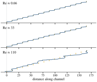
Because every stroke pushes fluid in only one direction, the nonlinear term \((u\cdot\nabla)u\) vanishes identically, so this too is an exact solution of forced Navier-Stokes. This time in a far different regime, with Reynolds number below 0.5 and forces some \(10^{11}\) times gentler than the main construction. We also checked it the hard way, with an independent spectral solver that integrates the full nonlinear equations from noisy initial conditions, and at gentle speeds it lands the answers within 0.02 lanes. Push it faster and it fails in a very physical way: past a Reynolds number of about 30, the shear layers between lanes go unstable and smear the answer.

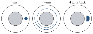
This multiplier has a deep limitation, though: its strokes all commute, so the order they come in doesn’t matter, and that rules out most interesting programs. Alternating the direction fixes this. Slide each row sideways by an amount that depends on which row it is, then each column by an amount that depends on which column it is, and you get a Feistel network, the same structure behind classic block ciphers like DES. Rounds like these can generate any even permutation of the cells,⁷ which in principle means any finite reversible program (given one spare bit). Our second flow uses this to encrypt a 16 × 16 grid of fluid cells. And because slow viscous flow is reversible, the decryption key is simply the same force, run backwards – the same effect behind G. I. Taylor’s famous demonstration of “unmixing” dye in a viscous fluid.⁸ In simulation, all 256 cells encrypt and return home, with forcing accurate to about half a percent.

More

For code, and a more in-depth technical explanation written by Claude Opus 5.5, check out the GitHub repo: github.com/RiScJ/ns-computer.