Electrodynamics simulation using the software package Meep
Originally written for PHYS 4410 (Advanced Experimental Physics) at Cornell University. Download the original paper (PDF).
Abstract. The fundamentals of electrodynamic simulation using the finite-difference time-domain method as implemented in Meep are explored. Two situations are considered as systems of study: a cavity resonator and a phased dipole array. I show how emergent properties of a system, such as quality factors, can be extracted for analysis; how visualizations can be readily created; and, describe potential future work with the software.
Introduction
The electromagnetic field has been chosen by humanity to be our primary means of communication. We use it to give us radio, television, the internet, and more. But as technology progresses, and the social demand for more powerful devices with greater throughputs and more innovative designs increases, so too does the need to be able to simulate and characterize these devices for iterative purposes.
Cellular modems, synthetic aperture radars, the new 5G NR – all of these technologies require materials having precise properties, and complex geometries. These things do not lend themselves easily to an analytical treatment, and so we must consider a method of numerical simulation. So much of the world revolves around these technologies and underlying computational processes that understanding those processes is critical toward understanding how the development of these technologies occurs.
Finite-difference time-domain
Meep simulates the electromagnetic field via a finite-difference time-domain (FDTD) method.1 In this method, Maxwell’s equations in space are discretized to a small cubic lattice. In this unit lattice, the components of the electric and magnetic fields are placed in a staggered fashion such that they do not overlap.2
The fields are stepped forward in time in an alternating manner – that is, first the electric fields are solved for, and the next time step the magnetic fields.2 This alternating pattern can be repeated to evolve the fields to an arbitrary desired future time.
Using an FDTD implementation such as Meep has certain benefits for simulating the electromagnetic field. For example, because this simulation method operates in the time domain, we can obtain information about the system’s response to a large bandwidth of frequencies in a single simulation run. In addition, we have full access to all components of the fields at any time; and, full and complete control of all material properties at every point in the simulated space, including high-order non-linearities.
While these benefits are noteworthy, there are also some weaknesses associated with FDTD. The most obvious of these is the large memory usage and simulation time associated with finely discretizing a three-dimensional volume of any significant size. This makes it computationally prohibitive to model geometries with fine features relative to the scale of the features of the field. There can also be numerical instabilities which arise from geometries failing to satisfy certain convergence conditions. Relating the two, far-field simulations are more likely to give rise to such instabilities, and take orders of magnitude longer to complete than near-field simulations.3
Of note is the fact that Meep handles all calculations in a system of natural units where \(\varepsilon_0=\mu_0=c=1\). I refer to such a unit system as Meep natural units, and abbreviate it as “MNU” in figures. It can be considered implicit in tables.
Cavity resonator
Meep has excellent documentation which includes a number of tutorial example simulations. Among them is the cavity resonator, which consists of a number of cavities spaced about a defect. I chose to use this tutorial as my introduction to the software because of its reach. That is, in the tutorial we learn how to run a simulation, how to extract meaningful data (like fluxes, quality factors, and resonant peak frequencies), how to visualize the data in a variety of ways (including animation of an arbitrary field component in time), as well as ways to construct the geometry programmatically.
The overall structure of simulation code using Meep takes roughly the same form as the following sparse example:
import meep as mp

# Define the constants we will need
resolution = 15 # (pxl / MNU)
freq = 0.7 # (c / a)

# Define the unit cell
cell = mp.Vector3(..., ..., ...)

# Define the sources
sources = [mp.Source(src= ...,
           center= ... ,
           component= ... ,
           amplitude= ...) for ... in ...]

# Define the geometry
geometry = [mp.Block(mp.Vector3(mp.inf),
            center= ... ,
            material=mp.Medium(
                epsilon= ...))]

# Define the perfectly matched layers
pml_layers = [mp.PML(1.0)]

# Define the simulation parameters
sim = mp.Simulation(cell_size=cell,
                    boundary_layers=
                      pml_layers,
                    geometry=geometry,
                    sources=sources,
                    resolution=
                      resolution)

# Run the simulation
sim.run(mp.to_appended('ez',
  mp.at_every(0.1, mp.output_efield_z)),
  until=30
)
This gives a general idea of the pattern that will be used across simulations: define any necessary constants; construct the unit cell; define and characterize the sources; define and characterize the geometry; create perfectly matched layers for the boundary; and, finally create the simulation object which links all the information together.
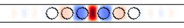
As an example, see figure 1 for a frame of an animation of a cavity resonator with \(N=3\) supporting one of its resonant modes. In this instance, the outer region does not support field propagation, and so rather nonphysically we see no losses to radiation.
Figure 2 shows a similar setup, but with \(N=16\). In addition, I have modified the surrounding region such that it has the properties of the vacuum. Here, we can see how some energy is lost as radiation to the surrounding space. Both figures show an arbitrary field component, with color conveying phase.
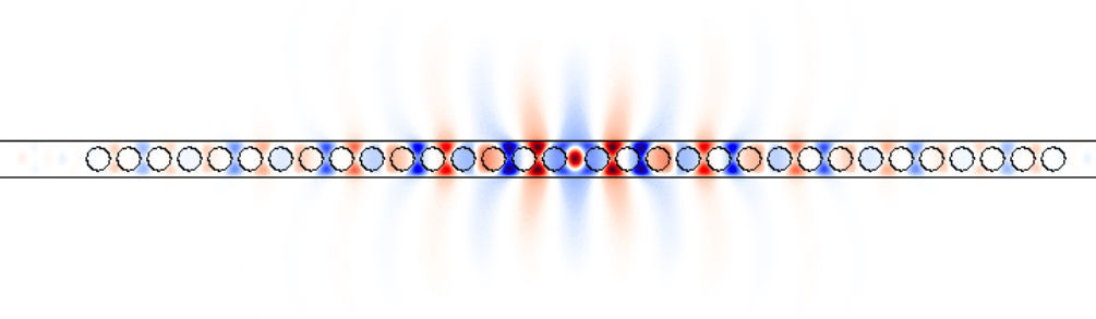
Moving from the first example to the second was a good experience in generating our geometry programmatically, taking much manual work away from the writer. Instead of being forced to write the location of each circular cavity individually, we take in the number of cavities on each side of the defect as a parameter, and construct the geometry in a for loop. This ability is very useful in general, and we will use the same technique when we later move to phased arrays.
While the ability to animate and visualize the results of a simulation may be visually appealing, they are useless as a calculation tool. It is therefore critical to be able to determine such things as the quality factors of resonances. Meep can do this readily as well. For the same cavity resonator shown in figure 2, see table 1 for a list of truncated values which contain information about the resonant modes that were detected for the system during the simulation.
| \(\Re[\omega]\) | \(\Im[\omega]\) | \(Q\) | \(\lvert A\rvert\) | \(\Re[A]\) | \(\Im[A]\) |
|---|---|---|---|---|---|
| 0.196 | 0.001 | -73.777 | 0.000 | 0.000 | 0.000 |
| 0.234 | -1.920 | 6105.959 | 6.044 | -3.998 | -4.533 |
| 0.312 | -0.000 | 323.178 | 0.010 | -0.010 | 0.001 |
| 0.325 | 0.000 | 322.428 | 0.102 | -0.053 | 0.087 |
Table 1. Resonant mode information for the cavity resonator pictured in figure 2, where \(\omega\) is the complex frequency, \(Q\) the quality factor, and \(A\) the complex amplitude.
The raw data output by the simulation is in the HDF5 format. The developers of Meep have likewise developed a set of tools which can be used to convert this HDF5 data into a variety of other formats. To produce an animation, for example, each of the timesteps is converted to a more traditional image format, such as PNG, and then a tool is used to stitch them together into a GIF or MP4, using something like ffmpeg. This ability to quickly render what the time evolution of some arbitrary field component looks like in time, on top of the physical underlying geometry, is one of the great strengths of FDTD methods. This makes this type of simulation very useful for communicating ideas to others quickly and easily.
The reason FDTD methods work so well for this type of task is because of the fact that they work in the time domain. There is no need to Fourier transform anything back from a frequency domain – we are already there. So we can simply display the raw data. It is noteworthy that this is a double-edged sword, however. As mentioned previously, this same advantage becomes a disadvantage if time-response information is what we are focused on.
After exploring the cavity resonator tutorial and concept to this point, I was satisfied with my understanding of the basics of the software and felt ready to implement my main goal of demonstrating rudimentary beamforming using a phased array of antennas.
Beamforming
To begin working with beamforming, it is simplest to start in two dimensions. The simplest radiators we can create would be dipoles. In Meep, we can model a dipole as an ideal sinusoidal current source with some complex amplitude and frequency. I choose to work with four of these dipoles here.
Because we are working in two effective dimensions, we can simply drop the third from our calculations and tell the software to model only an infinitely-thin region of space. This saves us a great deal in computation time.
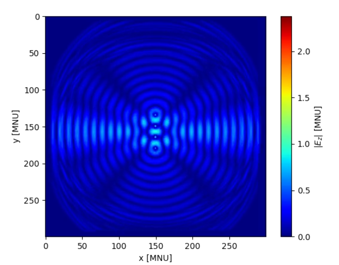
The dipoles are placed at half-wave intervals from one another, such that they are colinear. The rest of space starts with zero field. See figure 3 for a view of the steady state near field. Another of the drawbacks of FDTD is the difficulty associated with simulating the far field of even mildly complex systems. Because the entire spacetime volume needs to be stepped through, expanding our dimensions outwards by even a small degree leads to massive increases in the number of computational steps required per timestep.
To show how a phased array system can rotate the main lobe of the radiation pattern, a phase difference must be created between the radiators. This introduces a new aspect of the simulation software, because we must be able to “step in” and change something partway through. Luckily, Meep allows for such things. In the main call to the simulation function, we are able to add a set of parameters which dictate functions to be called under certain conditions. One of these conditions is the simulation time – we are able to call functions at a certain timestep, continuously after a certain timestep, continuously before, and so on. In the functions we call, we may modify anything we wish about the simulation: its geometry; the properties of the materials; or, as in our case, the properties of the sources. The modifications amount to this:
def phase_shift(sim):
    sim.change_sources([ ... ])

sim.run(mp.at_time(10, phase_shift), ...)
The modification will cause each dipole to accumulate an additional constant phase shift in addition to that accumulated by the one “before” it. After running the simulation with this new phase shift, we are able to view the effect on the main lobe of the radiation pattern. However, before once again looking at the steady state, it seems worthwhile to note how chaotic the transient patterns are immediately after the phase shift, as is shown in figure 4.
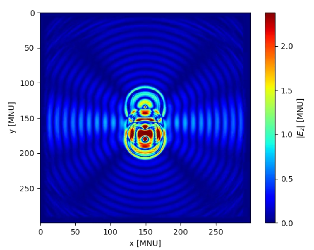
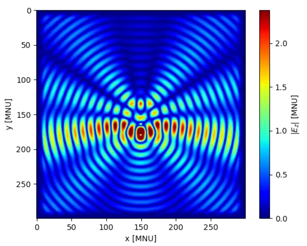
Lastly, we can observe the radiation pattern again once steady state is reached, as shown in figure 5. Compared with figure 3, there are a few significant differences. First, we can see a clear downward angle in the main lobes that did not exist prior to the phase shift. Secondly, not only has the radiation pattern rotated – the strength of the main lobe has actually increased dramatically. This ties into the third observation, which is that a null has formed above the array, opposite to the direction in which we have on average directed more energy. This makes sense – by directing more energy in the negative \(y\) direction, we must direct less in the positive \(y\) direction. This both acts to rotate the radiation lobes as well as to create the null in the pattern.
Discussion
Using the simulation software has already revealed some things which were unexpected. For example, I did not anticipate the behavior of the phase-shifted radiation pattern in my dipole array work above. I expected only rotation, and similarly, no additional null. But after more thought, both of these observations seem to be sensical. In this way, the software simulation of different environments is almost akin to a form of genuine experimentation. Because the FDTD method replicates real-world results in the overwhelming majority of situations, one could learn a significant amount about the real world from “playing” around in the simulation.
One could even imagine using the visualization abilities to gain physical intuitions for things which are traditionally difficult to explain or consider, such as the actual changes caused to a system by the presence of higher-order non-linearities.
For these reasons, I think the visual nature of simulations of this sort would lend themselves well to classroom settings. It would offer students a chance to not only better intuitively understand certain phenomena, but also a chance to explore on their own. FDTD methods have utility outside of engineering design and academic investigation. I think integrating the method into a more user-friendly interface and making the tools generally more accessible to the average person would be worthwhile.
Future work
The ability to utilize electrodynamics simulation software like Meep opens many potential avenues for future work. It becomes possible to study, concretely, the entire scope of electromagnetic design – from radiofrequency antennas to optical metamaterials.
Options are available for a future project to undertake as part of the lab. One potential idea is utilizing the software package to design a metamaterial antenna for the WiFi/BLE frequency band. This falls within the regime of possibility due to the ease of manufacture of PCB patch antennas at this wavelength, coupled with my previous experience with RF design. It would be interesting to manufacture such a device and compare its surface utilization and efficiency with some off-the-shelf component, such as a standard ceramic antenna.
Likewise, it would be possible to use the software package to model a phased-array system in the same frequency regime. This links more directly with the work shown here, but physical implementation is likely to be more involved. A simple array of patch antennas is likely to be simplest. A rasterscan approach could be utilized to roughly characterize the farfield pattern produced by the device, for example.
Lastly, as mentioned in the discussion, one could encapsulate FDTD as implemented by Meep into a more accessible and easier-to-use application, such as a web app. One could imagine a web interface where a user can graphically interact with the geometry, such as by dragging around pre-defined elements like blocks or spheres. Sources could be added in a similar fashion.2026 note. I went on to build exactly this: an interactive in-browser FDTD simulator. See the Maxwell project.
-
A. F. Oskooi, D. Roundy, M. Ibanescu, P. Bermel, J. D. Joannopoulos, and S. G. Johnson. Meep: A flexible free-software package for electromagnetic simulations by the FDTD method. Computer Physics Communications, 181(3):687–702, 2010. ↩
-
K. Yee. Numerical solution of initial boundary value problems involving Maxwell’s equations in isotropic media. IEEE Transactions on Antennas and Propagation, 14(3):302–307, 1966. ↩↩
-
A. Taflove and M. E. Brodwin. Numerical solution of steady-state electromagnetic scattering problems using the time-dependent Maxwell’s equations. IEEE Transactions on Microwave Theory and Techniques, 23(8):623–630, 1975. ↩
Errata
- 2026-06-05 — Corrected three typos present in the original (“underling” → “underlying”; “Is it noteworthy” → “It is noteworthy”; “signficant” → “significant”). The PDF preserves the paper as submitted.