Characterization of a microwave cavity resonator
Originally written for PHYS 4410 (Advanced Experimental Physics) at Cornell University. Download the original paper (PDF).
Abstract. A microwave cavity resonator is characterized through measurements of intra-cavity power, alongside forward and reverse powers in the feeding waveguide under various coupling configurations. A configuration is found which brings the cavity into resonance, and the resonant frequency and linewidth are determined. The quality factor is computed from these data, as well as a full description of the standing wave ratio as a function of frequency. The internal electric field magnitude is determined through a perturbative method.
Introduction and setup
Resonance is a phenomenon which presents itself in different ways across many different fields of study. Presented here is an investigation into the microwave-frequency resonant properties of a rectangular cavity resonator. The full microwave circuit begins with an oscillator. The oscillator produces a stable output-frequency continuous wave, dependent on the value of a given input voltage. The output wave frequency varies linearly with the input voltage. The oscillator output is immediately coupled into a waveguide via coaxial cable. The waveguide leads to a frequency-dependent attenuator. The attenuator introduces a power drop at the frequency it is tuned to. From the attenuator, the signal is again coupled into a waveguide which contains a directional coupler. The directional coupler has BNC terminations for both the forward and reverse powers. After the coupler, the signal is finally coupled into the cavity resonator, through an “iris”. The iris is a thin metal plate with a circular aperture in its center. There are multiple apertures with a range of diameters. Finally, the rear of the cavity resonator has variable effective length, due to a micrometer-controlled short.
A function generator is used to provide the voltage modulation that will serve as control input to the oscillator. A MiniCircuits ZX47-40 powermeter is used to transduce RF power levels to voltages. An oscilloscope is used to take readings of both of these signals. The cavity resonator has holes drilled through it at different positions along its length. A sapphire rod will be placed through these holes as a method of perturbing the internal cavity field.
Establishing resonance
To begin, the variable short at the end of the cavity is removed and replaced with a fixed back. The function generator is set to sweep in a sawtooth pattern with amplitude \(8\,\mathrm{V}\) and offset \(-2\,\mathrm{V}\), to generate a frequency raster. The output is split in two, and sent to both the oscillator and the oscilloscope’s first channel. The second oscilloscope channel is attached to the cavity’s BNC tap through the powermeter. In XY mode, the trace now represents a frequency response curve for the resonator. I save oscilloscope traces captured via this method to a flash drive. Next, the powermeter is detached from the cavity’s BNC tap and attached to the reverse power tap of the directional coupler. The trace now shows the frequency-dependent reflected power. The trace is similarly written to flash storage. Finally, the powermeter is connected to the forward power tap of the directional coupler. This trace shows the power coming from the oscillator, and is also saved. This process is repeated for the different available coupling irises.
Of the tested irises, in the configuration without the variable short, I was unable to bring the cavity into resonance. Because of this, there are no meaningful data to report (such as center frequencies or linewidths, etc.).
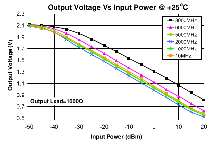
The variable short is replaced. Similarly, no resonance is attained for any of the coupling irises save for with diameter \(D=10.5\,\mathrm{mm}\). With the micrometer brought to a reading of \(5.64\pm0.01\,\mathrm{mm}\), the cavity is brought into resonance. In order to calibrate frequency values, it is necessary to use the attenuator. Through careful positioning of the attenuator, a visible dip is brought into the power spectrum. The dip is moved to an arbitrary voltage, which is read off. The corresponding frequency is then read from the attenuator. This is done again to provide a calibration scale. Here, I find \(0.00 \pm 0.02\,\mathrm{V}~\to~8445.0\pm0.1\,\mathrm{MHz}\), and \(2.00\pm0.02\,\mathrm{V}~\to~8454.5\pm0.1\,\mathrm{MHz}\). Likewise, a calibration curve is required for the powermeter. One can be found from its datasheet,1 and is available in figure 1. The curve was modeled in analysis as a line fitting the points \((0\,\mathrm{dBm},~1.3\,\mathrm{V})\) and \((-27\,\mathrm{dBm},~1.9\,\mathrm{V})\).
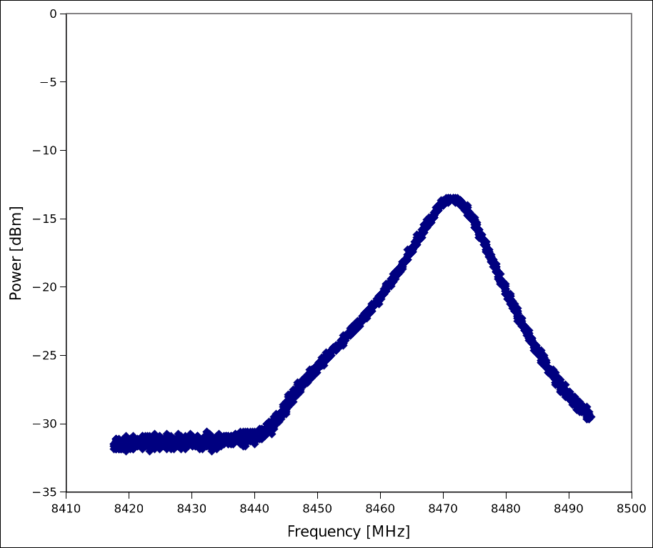
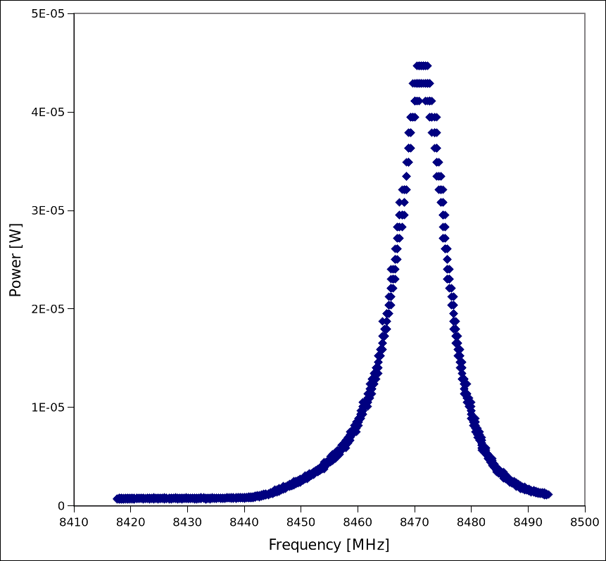
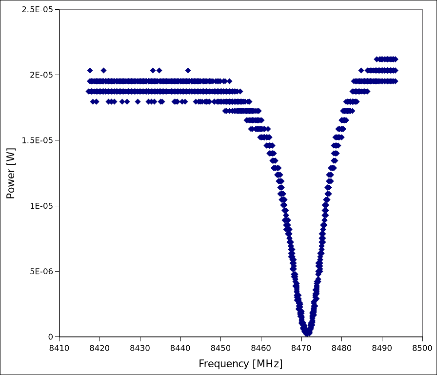
The frequency response for the cavity is visible in figure 2, in milliwatt-referenced decibels. The resonant peak is prominent. Figure 3 shows the same curve in watts. The cavity attains a peak power of \(P_0=(4.46\pm0.01)\times10^{-5}\,\mathrm{W}\) at a frequency of \(f_0=8471.7\pm0.1\,\mathrm{MHz}\). The linewidth is measured to be \(\delta f=10.2\pm0.2\,\mathrm{MHz}\), which when combined with the center frequency gives a quality factor of \(Q=830.5\pm16.3\).
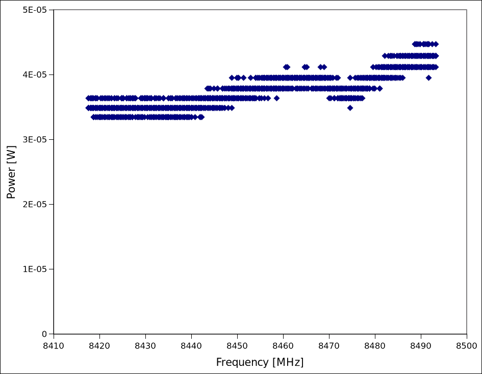
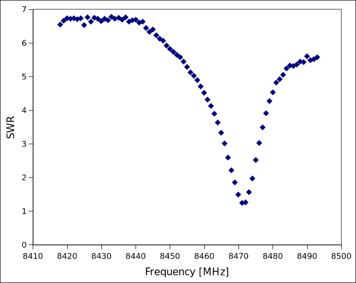
The forward and reverse powers are plotted in the same fashion, and are seen in figures 4 and 5, respectively. To determine robustly the quality of the impedance match, it is beneficial to calculate the standing wave ratio:
$$\mathrm{SWR}=\frac{1+\sqrt{P_r/P_f}}{1-\sqrt{P_r/P_f}}$$
where \(P_r\) and \(P_f\) are the reverse and forward powers, respectively.
The result over all frequencies can be seen in figure 6. The best match is an SWR of \(1.20\pm0.1\) at a frequency of \(f_0=8471\pm1\,\mathrm{MHz}\), which is in excellent agreement with the other methods of measuring the center frequency. This corresponds with a reflection coefficient of roughly \(\Gamma\approx0.09\).
Internal electric field
The previous methodology for collecting frequency response curves is performed again. This time, a sapphire rod is inserted into one of thirteen holes which span the length of the cavity resonator. For each sample, the new center frequency is found, and the difference between it and the unperturbed center frequency, \(\Delta f\), is found. Labeling the 11 colinear rod positions by an integer incrementing from the left, and the “vertically” displaced rod positions by “up” and “down” – for positions 2, 3, 7, 8, and 11, no meaningful \(\Delta f\) could be found. This is because inserting the rod into this position appears to collapse the resonance altogether. Because of this loss in information about the internal field distribution, I decided to simply average the shifts together. This would give information about the average electric field strength, and it will still be possible to recover modal information from other arguments. The average frequency shift from rod insertion comes to be \(22\pm0.5\,\mathrm{MHz}\).
The relative frequency shift is related to the internal electric field, and internal energy, by the following expression:2
$$\frac{\Delta f}{f}=\frac{1}{4U}\int_\mathcal{V}\mathrm{d}^3r~\varepsilon|E|^2$$
where \(U\) is the total internal energy of the cavity, \(\mathcal{V}\) is the perturbation region (here, the volume of the rod), \(\varepsilon\) is the permittivity of the unperturbed medium, and \(E\) is the unperturbed electric field strength. This expression can be further simplified. Because the rod perturbation method inherently averages the field over its length anyway, we can simply replace the integration with a multiplication by the rod’s volume:
$$\frac{\Delta f}{f}=\frac{1}{4U}\pi r^2h\varepsilon|E|^2$$
where \(r\) is the radius of the sapphire rod, and \(h\) is the height of the cavity. This can be rearranged to give a form for the average electric field magnitude:
$$E=\sqrt{\frac{4U\Delta f}{\pi r^2h\varepsilon f}}$$
A form is still required for the total internal energy. We can get one from one of the definitions of the quality factor:
$$U=\frac{QP}{2\pi f}$$
which for this cavity comes to be \((6.96\pm0.15)\times10^{-13}\,\mathrm{J}\). Interestingly, this is an incredibly small amount of energy, but still corresponds to an expected \(1.24\times10^{11}\) photons in the cavity at any moment. For the cavity height, \(h=10.3\,\mathrm{mm}\). The rod has radius \(r=0.675\,\mathrm{mm}\). So, we can compute the average field strength, and find it to be \(E=235.3\,\mathrm{V}\,\mathrm{m}^{-1}\).
Although through the averaging technique modal information of any kind has been lost, it is simple to calculate the cutoff frequencies for the TE and TM modes of a rectangular waveguide, and gain information in this manner. Because TE and TM modes have the same cutoff frequencies for a rectangular waveguide, it is only necessary to check one. We have:
$$f_c=\frac{c}{2}\sqrt{\left(\frac{m}{a}\right)^2+\left(\frac{n}{b}\right)^2}$$
is the cutoff frequency for mode \(\mathrm{TE_{mn}}\), for major axis \(a\) and minor axis \(b\), and their corresponding nodal counts \(m\) and \(n\), respectively. For this cavity, some approximate values are listed in table 1.
| Mode | \(f_c\) [GHz] |
|---|---|
| \(\mathrm{TE_{10}}\) | 6.56 |
| \(\mathrm{TE_{01}}\) | 14.5 |
| \(\mathrm{TE_{11}}\) | 16.0 |
Table 1. Approximate cutoff frequencies of cavity modes.
The only candidate modes are then \(\mathrm{TE_{10}}\) or \(\mathrm{TM_{10}}\), by cutoff frequency alone. However, magnetic modes in nonmagnetic media are only allowed for both nonzero \(n\) and \(m\). Because \(n\) here is zero, the cavity must only be supporting the \(\mathrm{TE_{10}}\) mode.
Conclusion
A cavity resonator was characterized through a variety of methods. Through switching out coupling irises, it was found the best impedance match is achieved with an iris of diameter \(10.5\,\mathrm{mm}\), and the variable short set to \(5.64\,\mathrm{mm}\). By calibrating frequencies with the variable attenuator, the resonant frequency was found to be \(8471.7\pm0.1\,\mathrm{MHz}\). Reflected power was found to be minimized at \(8472\pm1\,\mathrm{MHz}\), in good agreement with the previous method. The quality factor was found to be \(830.5\pm16.3\), demonstrating a reasonably good quality resonator. The standing wave ratio was also found to be minimized at \(8471\pm1\,\mathrm{MHz}\), another measurement in agreement with the previous. It attains a minimum value of \(1.20\), agreeing with the quality factor in representing a reasonably good quality resonator. Finally, the average internal electric field strength was found to be \(235.2\,\mathrm{V}\,\mathrm{m}^{-1}\).
Errata
- 2026-06-05 — Corrected three typos present in the original (“center frequenies” → “frequencies”; “are are seen” → “and are seen”; “pertubation” → “perturbation”) and a missing terminal period. The PDF preserves the paper as submitted.